

TEXT TO COLUMNS EXCEL FUNCTION - THE ULTIMATE GUIDE
There are times when you need to export data from an application or software to Excel. The data appears to be continuous, and you want to separate it into different columns. You will need the Text to Columns function for this.
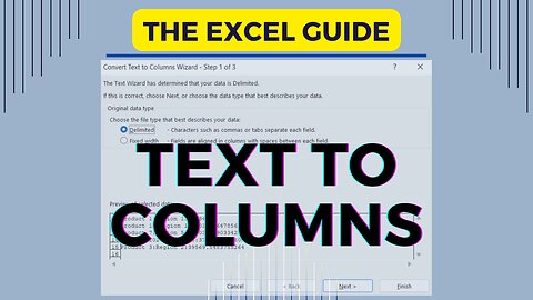
Text to Columns in Excel is a method used to separate a text into different columns. There are two options to use Text to Columns in Excel:
1. Delimited which is good if there is a common character like tab, semicolon, comma, space or other characters that can be used to separate the texts.
2. Fixed Width which is ideal if the fields of your data are aligned in columns.
You can quickly show the Text to Columns window with a keyboard shortcut. Watch this video to learn about it.
TITLE: TEXT TO COLUMNS EXCEL FUNCTION - THE ULTIMATE GUIDE
#texttocolumns #exceltutorial #howtodotexttocolumnsinexcel #keyboardshortcut
12
views
HOW TO INSERT MULTIPLE ROWS AND COLUMNS
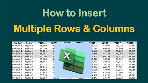
Inserting rows or columns in Excel is one of the most basic and repetitive tasks you’ll need to do. Adding one is quick and easy. But what about if you need to add multiple rows or columns? What if you need to add hundreds or thousands of rows or columns?
In this video, you will learn how to insert multiple rows or columns using the basic way and using the keyboard shortcut to make it fast. And both ways are easy to do.
TITLE: HOW TO INSERT MULTIPLE ROWS AND COLUMNS
#insertrows #insertcolumns #insertmultiplerows #insertmultiplecolumns #waystoinsertrowsandcolumns
8
views

MS EXCEL TUTORIAL: TIPS TO QUICKLY HIGHLIGHT CELLS AND NAVIGATE THE TABS
Highlighting cells in Excel can be much faster using some simple shortcut keys. You can quickly select and highlight multiple cells in a contiguous range with the use of 3 shortcut keys – control, shift and arrow.
Watch this video to know how. Plus you will also learn how to swiftly navigate the tabs without using a mouse.
TITLE: TIPS TO QUICKLY HIGHLIGHT CELLS AND NAVIGATE THE TABS
#exceltutorial #excelkeyboardshortcut #exceltips #quicklyhighlightcells #quicklynavigatethetabs
11
views
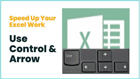
MS EXCEL TUTORIAL: HOW TO NAVIGATE THE WORKSHEET QUICKLY
Excel has a lot of features that can make you work faster and easier. This includes navigating around a large worksheet. Excel allows you to move around quickly. The secret is simply with the use of CTRL and ARROW. This video will quickly guide you on how to do it.
TITLE: HOW TO NAVIGATE THE WORKSHEET QUICKLY
#howtonavigatequickly #exceltutorial, #exceltraining
20
views
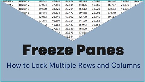
MS EXCEL TUTORIAL: HOW TO FREEZE MULTIPLE ROWS AND COLUMNS
When you are working on a large set of data, and you want to retain the top row header, or the left column header when you scroll down or to the right, freeze panes function is the answer.
You can keep an area of a worksheet visible while you scroll to another area by using the Freeze Panes Excel function under the View tab. With this, you can lock specific rows and columns in place. Just go to the cell below the rows and to the right of the columns you want to keep visible when you scroll and click Freeze Panes.
This video also includes a keyboard shortcut for you to be able to do it swiftly.
Title: How to Freeze Multiple Rows and Columns
#freezepanes #freezemultiplerows #freezemultiplecolumns #keyboardshortcut #exceltip
36
views

MS EXCEL TUTORIAL: THE COUNTBLANK AND COUNTA EXCEL FORMULAS
COUNTBLANK and COUNTA are very straight forward and easy-to-use excel functions and are both used to count a range of cells. The difference? COUNTBLANK is a premade Excel function used to count the number of empty cells in a given range. It returns a count of empty cells in a range.
Title: MS Excel Tutorial - The COUNTBLANK and COUNTA Excel Formulas
#countblank, #counta, #excelfunctions, #excelformula
12
views

EXCEL TUTORIAL - WHEN TO USE THE IFISBLANK FORMULA
IFISBLANK is an alternative to the ISBLANK formula. The ISBLANK formula displays the answer true or false if the value is empty of not. If you want other answers to display instead of just true or false, IFISBLANK is the ideal formula to use.
By adding IF to the ISBLANK formula, you will have more options on how to display the answer, so that it will be easy for you to read and understand the data.
Title: Excel Tutorial - When to Use the IFISBLANK Formula
#IFISBLANK, #exceltutorial, #excelonlinetraining, #microsoftexcelfunction, #microsoftexcelformula, #microsoftexcelcommand, #microsoftexceltips
10
views
HOW TO USE ISBLANK IN EXCEL
The easy way to spot blank cells is through the ISBLANK formula. It is used to check whether a cell is empty or not and returns true or false. It shows true if the cell is empty, and false if it contains data.
ISBLANK function is so easy to use. You can find it within the information group under Formulas tab.
Title: How to Use ISBLANK in Excel
#ISBLANK #excelfunctions #exceltutorial #howtouseisblank
8
views

HOW TO QUICKLY REMOVE DUPLICATES IN EXCEL
If you want to remove duplicates from a set of data, you don't have to check them one by one. Excel has a great tool that can help you do this in such a quick manner. You can make use of the Remove Duplicates function in the data tools under the Data menu.
This video introduces the keyboard shortcut so that you won’t have to go to go through the tabs to click. With just a few keys to type, the Remove Duplicates window appears where you can choose options on how to perform the function.
Watch this video and see the complete guide.
TITLE: HOW TO QUICKLY REMOVE DUPLICATES IN EXCEL
#removeduplicatesinexcel #keyboardshortcut #exceltips
9
views
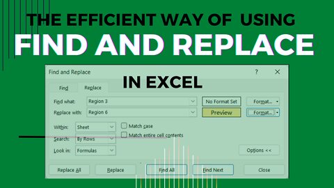
HOW TO QUICKLY FIND AND REPLACE DATA IN EXCEL
Sometimes you need to find a word or number somewhere in your spreadsheet, and replace it with another value. Excel’s Find and Replace can do this instantly, even from a large amount of data. The process can be even faster with the use of the keyboard shortcuts included in this tutorial.
Watch this video and find out.
Title: How to Quickly Find and Replace Data in Excel
#excelfunctions #exceltutorial #microsoftexcel #findreplacedatainexcel
16
views

EXCEL PASTE SPECIAL OPTIONS AND SHORTCUT KEYS
The video shows the useful functions of Paste Special in Excel and how to make the process faster by using keyboard shortcuts to paste the commonly used paste special elements like values, formats, subtract and transpose. There are more options to choose like paste comments, validation, all using source theme, all except borders, column widths, formulas and number formats as well as values and number formats. There are also other operations that Excel can do with the copied data like add, multiply and divide. And you have the option to skip blanks when you paste the copied cells.
All of the Paste Special commands work within the same worksheet as well as across different sheets and workbooks.
Title: Excel Paste Special Options and Shortcut Keys
#pastespecial #shortcutkeys #keyboardshortcut #exceltips
20
views

ABSOLUTE CELL REFERENCE IN EXCEL
Absolute Cell Reference is the answer if your formula needs to refer to a fixed location or fixed cell reference or to lock the reference in the formula.
In Excel, Relative Cell Reference is the default reference type. When you copy a formula to another cell, it changes based on the relative position of the row or column. In order to fix a reference, you should use the Absolute Cell Reference.
Title: Absolute Cell Reference in Excel
#absolutecellreference #fixedcellreference #howtofixtheexcelformula
6
views
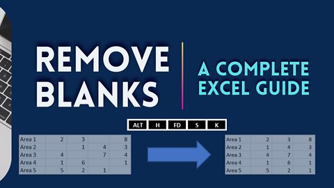
3 WAYS TO REMOVE BLANK CELLS OR EMPTY CELLS
This video will guide you on how to remove blank cells or empty cells from selected range of data.
The first thing to do is to highlight the range of cells. If you want to select all cells with data, click anywhere in the table and press CTRL + A.
When you have selected the data range, you can now go to the Data tab where Go To Special Excel function can be found. This video will show the detailed way of doing it as well as the keyboard shortcuts to speed up the process.
The 2nd method to remove blank cells is through the keyboard shortcut ALT – H – FD and the 3rd one is a shorter way to do it. It’s though the F5 key. Just one click and Go To window where you can select Special is right in front of you.
After watching this, you will learn or be guided with the complete process of removing blank cells.
Title: 3 Ways to Remove Blank Cells or Empty Cells
#removeblankcellsemptycells
#howtoremoveblankcellsemptycells
#keyboardshortcuttoremoveblankcellsemptycells
#gotospecialexcelfunction
11
views

THE BASIC WAYS TO FILTER DATA IN EXCEL
If you want to display only selected info from a set of data, you can do it fast with Filter in Excel. This function filters data based on certain criteria that you define. Watch this video presenting the basics of this Excel function.
Title: The Basic Ways to Filter Data in Excel
#exceltutorial #excelonline #filterdata #keyboardshortcuts #excelguide
9
views

HOW TO SET DATA VALIDATION RULES
You can control the type of data to be entered into your worksheet with the use of Data Validation in Excel. This video will show you how to set validation rules.
Excel Data Validation allows you to limit data entries to the dropdown list and restricts data outside of the range. There are eight options available to validate the input:
1. Any Value – this is the default if no validation rule is set.
2. Whole Number – if data entry is limited to whole numbers or only whole numbers are allowed. If this validation rule is selected, other validation options have to be defined to further limit the input, such as between, not between, equal to, not equal to, greater than, less than, greater than or equal to and less than or equal to.
3. Decimal – is similar to Whole Number option but allows decimal values within the range given.
4. List – allows only values from a predefined list and presented to the user as a dropdown menu control.
5. Date – only dates are allowed.
6. Time – data entry is limited to times only.
7. Text Length – validates entry based on the number of characters or digits.
8. Custom – validates input using a custom formula.
This function can be found under the Data tab and the keyboard shortcut for this Excel function is also introduced in this video.
Title: How to Set Data Validation Rules
#datavalidation #howtosetdatavalidationrules
8
views
HOW TO QUICKLY MOVE DATA
There’s a smart trick to move data to another place in Excel without using cut and paste.
The most common way to move data is to use cut and paste functions. For this method, you have three options to do it - the cut and paste buttons on the ribbon, the keyboard shortcuts control-x to cut and control-v to paste, and the right-click menu.
There’s a quick method to move data without the need of cut and paste functions. You just need to highlight and drag. Highlight the cell/s, column/s or row/s to be moved, then drag the border to another location. That’s it.
You don’t have to go through the long process for this simple excel activity. Master the quick method to move data and you will save a lot of time.
Title: How to Quickly Move Data
#exceltipsandtricks #quicklymovedata #exceltutorial #learnexcel #quicklymovedata
33
views

EXCEL AUTO-FIT: THE FASTEST WAY TO ADJUST ROWS AND COLUMNS
Excel Auto-Fit is the easiest and fastest way to adjust the width of the column/s and the height of the row/s. Just double click the border and you’ll get what you want.
Using this Excel function will automatically adjust the column and row to fit the whole text. This can be applied to a single or multiple columns and rows.
After watching this video, you’ll be able to save a lot of your precious time when working with Excel.
Title: Excel Auto-Fit: The Fastest Way to Adjust Rows and Columns
#excelautofit #fastestwaytoadjustrowsandcolumns #excelshortcut #exceltip
6
views
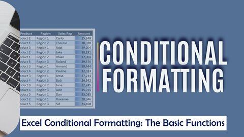
THE AWESOME FEATURES OF CONDITIONAL FORMATTING IN EXCEL
Conditional Formatting offers various formatting options. This video presents several basic features of Conditional Formatting Excel function. It’s a great way to quickly visualize data in a spreadsheet.
With its keyboard shortcut, you’ll be instantly presented with the window that allows you to:
• Highlight cells based on condition
• Set top/bottom rules and highlight the data covered by the rules
• Access various options for data bars, color scales and icon sets
• Set a new rule or condition
Watch this video and take your Excel skills to the next level!
Title: The Awesome Features of Conditional Formatting in Excel
#conditionalformatting #formattingtechniques #shortcutkeys #exceltips #excelshortcuts #
14
views
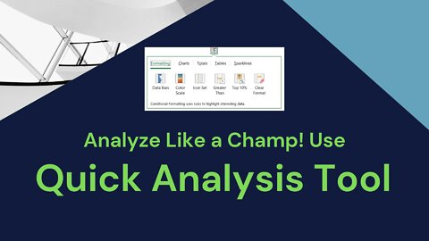
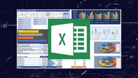
USE QUICK ANALYSIS TOOL TO ANALYZE LIKE A CHAMP IN EXCEL
This video features the uses of Excel’s Quick Analysis Tool and illustrates how you can use it. This tool is like a Swiss Knife of data analytics filled with powerful tools to help you manage your data sets of any size. Here we can do quick formatting to add visual representation, and help identify distinct figures like the highest and the lowest. It includes charts, color coding and formulas.
Just one click of the Quick Analysis button uncovers the following tools to analyze or format your data:
• Formatting Tools
o Data Bars
o Color Scale
o Icon Set
o Greater Than
o Top 10%
• Charts
o Clustered Column
o Clustered Bar
o Line
o Pie
o Scatter
o Other Recommended Charts
• Totals (Rows and Columns)
o Sum
o Average
o Count
o % Total
o Running Total
• Tables
• Sparklines
All of those functions are in one button found at the bottom right corner of the highlighted data.
Title: Use Quick Analysis Tool to Analyze Like a Champ in Excel
#quickanalysistool #excelformatting #excelshortcuts #excelanalysis
23
views
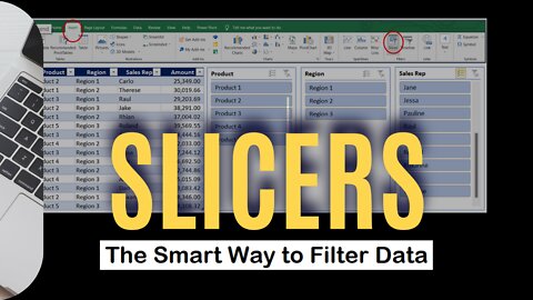
EXCEL SLICERS - THE SMART WAY TO FILTER DATA
In this video, you will learn how Slicers in Excel can help you filter large amount of data in such a cool and fast way.
Slicers in Excel are used along with Excel tables or pivot tables. Aside from filtering the data, slicers also help you with an easy understanding of the information being extracted and displayed on the screen. On top of that, the slicers are nice to look at so it’s a combination of art and competence. It’s a sophisticated, yet so easy-to-use excel function. Another benefit is that Excel Slicers help in maintaining data security and integrity as the user is only interested in filtering and using the necessary information and avoid ruining the actual data. To make it even faster for you to put this function in place, keyboard shortcuts are included in the illustration of this video.
Watch this video for more details.
Title: Slicer-The Smart Way to Filter Data in Excel
#excelslicers #filterdata #smartwaytofilterdata #exceltips
14
views
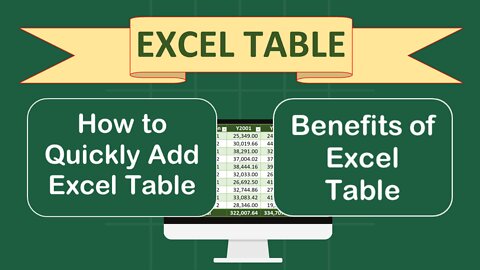
8 AMAZING BENEFITS OF USING EXCEL TABLE
This video showcases the useful features of Table in MS Excel. After watching this, you’ll find out that Table does not only organize and structure your data. It also helps to expedite your work in many ways.
With just two clicks of the keyboard shortcut, you’ll have a formatted table for your data.
As soon as you have the table, you can do the following:
• Easily filter the information that you want to display.
• Quickly add or remove rows or columns with the use of the resize handle that comes along with the table.
• Automatically add a formatted column when you type a text right beside the table and a formatted row when you type a text right below the table.
• Quickly transfer the whole table.
• Create a formula in one cell and automatically fill the other cells in the column with the same formula.
• Display a drop-down list of various commonly used formulas or calculations by creating one formula right below the table. With the drop-down list, you can easily do other calculations.
• Swiftly hide or show the row containing the total.
• Easily change the format or choose other formatting options.
So, this one excel function can offer you several ways to expedite you work and at the same time help you create a high-level report.
Watch and try it!
34
views