

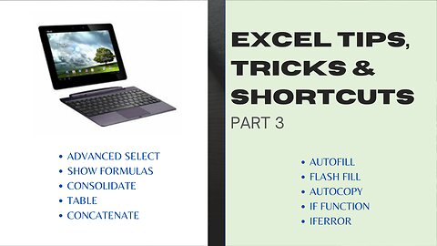
Excel Tips, Tricks and Shortcuts Part 3: The Functions You Need to Know
This video introduces another 10 advanced excel functions. Explore these amazing Excel functions that will elevate your data manipulation and analysis skills. Get ready to unlock the full potential of Excel!
1. ADVANCED SELECT: This function is useful to instantly find and select the items that you need. It includes the keyboard short-cuts to quickly display the function’s window.
2. SHOW FORMULAS: Learn how to display the actual formulas in cells instead of their results. This feature is invaluable for auditing and understanding complex calculations.
3. CONSOLIDATE: It’s an excel function that is used to consolidate data from one workbook, or from different open workbooks. Understand how to merge data from multiple ranges or worksheets into one, simplifying your analysis and reporting tasks.
4.TABLE: Excel table comes with useful features. It does not only organize and structure your data. It also helps to expedite your work in many ways. Here are the 8 benefits of using Excel Table:
• Easily filter the information that you want to display.
• Quickly add or remove rows or columns with the use of the resize handle that comes along with the table.
• Automatically add a formatted column when you type a text right beside the table and a formatted row when you type a text right below the table.
• Quickly transfer the whole table.
• Create a formula in 1 cell and automatically fill the other cells in the column with the same formula.
• Display a drop-down list of various commonly used formulas or calculations by creating 1 formula right below the table. With the drop-down list, you can easily do other calculations.
• Swiftly hide or show the row containing the total.
• Easily change the format or choose other formatting options.
5. CONCATENATE: There are 3 ways to combine two or more text strings and place them together in 1 cell:
• With the use of the Concatenate Excel formula.
• Through the Textjoin function which concatenates a list or range of text strings using a delimiter.
• With the use of &.
6. AUTO FILL: Used to automatically fill the remaining cells based on the pattern of what was entered.
7. FLASH FILL: Designed to do automatic entry of data. What you do to the first cell will be done to the remaining cells with the use of this function. You just have to enable it through the box for Automatically Flash Fill.
8. AUTO COPY: Used to automatically copy the formula down with just a simple double click at the lower right corner of the cell with formula.
9. IF FUNCTION: There are various logical tests that can be done with the use of the If function. It is used to evaluate data in the spreadsheet. IF Excel function determines whether the logical test is true or false, and it displays a certain value as defined in the formula. It is also helpful if you want to hide formula error from your spreadsheet.
30. IFERROR: This is similar to the IF function which eliminates or hides an error if the function does not suit the given data. You can choose what to be shown in case of an error or if the formula is not applicable. This is a faster way to avoid displaying error.
Title: Excel Tips, Tricks and Shortcuts Part 3: The Functions You Need to Know
0:00 Introduction
0:29 ADVANCED SELECT
1:00 SHOW FORMULAS
1:35 CONSOLIDATE
4:17 TABLE
8:11 CONCATENATE
10:49 AUTO FILL
11:28 FLASH FILL
12:15 AUTO-COPY
12:36 IF FUNCTION
14:26 IFERROR
#exceltipstricksshortcuts
#advancedselectinexcel
#showformulasinexcel
#consolidatedatainexcel
#exceltable
#howtocombinetextstrings
#excelautofill
#excelflashfill
#excelautomaticcopy
#ifexcelfunction
#iferrorexcelfunction
150
views
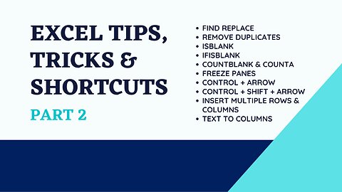
Excel Tips, Tricks and Shortcuts Part 2: Efficient Data Management
In this video, we'll explore ten powerful Excel functions that will take your data management and analysis skills to the next level. Let's dive right in!
1. Find Replace: Discover how to quickly find specific values in your spreadsheet and replace them with new ones. This function saves you time when updating or correcting large datasets.
2. Remove Duplicates: Learn how to efficiently remove duplicate values from your data, ensuring data accuracy and avoiding redundancy.
3. ISBLANK: Understand how to use this function to check if a cell is empty or blank. It's a handy tool for conditional formatting or data validation purposes.
4. IFISBLANK: Explore how to combine the IF function with ISBLANK to perform different actions based on whether a cell is blank or not. This function adds flexibility to your data manipulation tasks.
5. COUNTBLANK and COUNTA: Master these two functions to count the number of blank cells or non-blank cells in a range. They provide valuable insights into the completeness of your data.
6. Freeze Pane: Discover how to freeze rows or columns in Excel to keep important headers or labels visible while scrolling through a large dataset.
7. CTRL and Arrow Combination: Unlock the power of keyboard shortcuts by learning how to navigate quickly to the last cell in a row or column with this time-saving combination.
8. CTRL, Shift and Arrow Combination: Combine the CTRL and Shift keys with the Arrow keys to select large ranges of data in Excel effortlessly.
9. Insert Multiple Rows and Columns: Learn how to insert multiple rows or columns at once, saving you from repetitive manual insertion.
10. Text-to-Columns: Uncover this powerful tool that allows you to split data in a single column into multiple columns based on a delimiter or fixed width.
By incorporating these functions into your Excel repertoire, you'll become a data management and analysis expert. Thank you for watching, and happy Excel-ing!
Title: Excel Tips, Tricks and Shortcuts Part 2: Efficient Data Management
#ExcelFunctions #ExcelTips #DataManagement #DataAnalysis #ExcelTricks #ExcelShortcuts #ProductivityHacks #DataManipulation #ExcelMastery #SpreadsheetSkills #FindReplace #RemoveDuplicates #ISBLANK #IFISBLANK #COUNTBLANK #COUNTA #FreezePane #ControlArrowCombination #ControlShiftArrowCombination #InsertMultipleRows #InsertMultipleColumns #Text-to-Columns
30
views
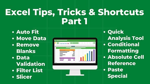
10 Excel Tips, Tricks and Shortcuts: Productivity Hacks Part 1
In this video, you will learn ten valuable Excel functions that will enhance your productivity and make your work much easier. It's the 1st part of a series of videos showing various basic to advanced excel tips, tricks and shortcuts. Let's dive right in!"
1. Auto Fit. Have you ever encountered cells that don't display the complete content? With Auto Fit, you can automatically adjust the column width and row height to fit the content perfectly.
2. Move Data. Learn how to swiftly move cells, rows, or columns to a different location. This function can save you a lot of time and effort.
3. Remove Blanks. Discover how to efficiently eliminate empty cells from your data range. This trick helps you streamline your spreadsheet and focus on the relevant information.
4. Data Validation. Learn how to set up rules and restrictions for data entry in specific cells. This feature is fantastic for maintaining data accuracy and consistency.
5. Discover how to filter and sort your data effectively, allowing you to quickly find what you need. Filtering saves you from scrolling through large datasets.
6. Slicer. Learn how to create slicers to filter data visually in tables. This handy tool provides a user-friendly way to analyze your data dynamically.
7. Quick Analysis Tool. Uncover this hidden gem that offers instant access to various data analysis options. It's a powerful feature for quick insights and visualizations.
8. Conditional Formatting. This function helps you highlight important information and visualize patterns in your data.
9. Absolute Cell Reference. Understand how to lock specific cells when copying formulas across different cells. Absolute cell references ensure your formulas always refer to the intended cells.
10. Paste Special. Master the art of pasting values, formulas, formatting, and more with precision. This feature enables you to control exactly what you paste in your worksheets.
By utilizing these functions such as Auto Fit, Move Data, Remove Blanks, Data Validation, Filter List, Slicer, Quick Analysis Tool, Conditional Formatting, Absolute Cell Reference, and Paste Special, you'll become an Excel pro in no time.
Thank you for visiting my channel. As a CPA, I have been working for more than 20 years and held various finance functions. Currently, I work as a Financial Consultant of a manufacturing company. Excel has been my tandem in my career and I'm happy to share my skills to you.
As a newbie in YouTube, any amount of support like your subscription to my channel is very much appreciated.
0:00 Introduction
0:23 AUTO FIT
0:58 MOVE DATA
1:27 REMOVE BLANK
2:09 DATA VALIDATION
3:40 FILTER LIST
4:27 SLICER
5:45 QUICK ANALYSIS TOOL
7:41 CONDITIONAL FORMATTING
9:45 ABSOLUTE CELL REFERENCE
10:46 PASTE SPECIAL
#ExcelTips #ExcelTricks #ExcelShortcuts #ProductivityHacks #DataManagement #SpreadsheetSkills #ExcelFunctions #DataAnalysis #ExcelMastery #ExcelEfficiency #AutoFit #MoveData #RemoveBlanks #DataValidation #FilterList #Slicer #QuickAnalysisTool #ConditionalFormatting #AbsoluteCellReference #PasteSpecial
Excel Tips, Tricks and Shortcuts That Make Your Life Easier
58
views

DO YOUR OWN FINANCIAL EVALUATION WITH PMT EXCEL FUNCTION
If you are planning to borrow money and would like to evaluate how much payment is required from you every period, there’s an Excel function that can help you. This Excel function allows you to determine the installment amount.
The Excel Payment or PMT function is a financial function that calculates the periodic payment for a loan based on constant payments and a constant interest rate. You can use the PMT function to figure out payments for a loan, given the loan amount, number of periods to pay, and interest rate.
In this video, I will show you how to do it.
Title: Do Your Own Financial Evaluation with PMT Excel Function
#pmtexcelfunction
#paymentexcelfunction
#howtocalculateloanamortization
#howtocalculateloanpayment
#financialfunction
89
views
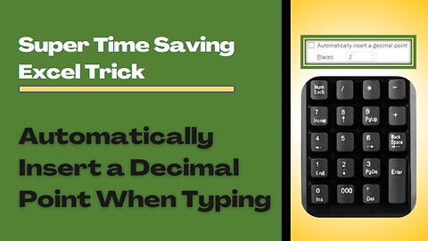
SUPER TIME-SAVING EXCEL TIP: AUTOMATICALLY INSERT A DECIMAL POINT WHEN TYPING
When manually entering data or numbers with decimal point, you can make the data entry faster by letting excel insert the decimal point for you, so you won't have to do it over and over again. This video presents a super time-saving excel tip - set to automatically insert a decimal point when typing.
Title: Super Time-Saving Excel Tip: Automatically Insert a Decimal Point When Typing
#automaticallyinsertadecimalpointwhentyping
#shortcutkeys
#keyboardshortcuts
#exceltricks
#exceltipsandtricks
#exceltutorial
23
views
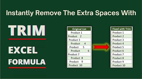
INSTANTLY REMOVE THE EXTRA SPACES WITH TRIM EXCEL FORMULA
TRIM excel function is great for organizing large amounts of data. Sometimes, your data contains extra spaces at the beginning, end or in between words within a cell. Aside from being difficult to read and understand, the data also looks untidy.
The good thing is that there’s a way to fix it and it can be done swiftly. Thanks to Excel’s TRIM function which removes those extra spaces, irrespective of the number of spaces that are there in that selected cell, with its, so easy-to-use formula.
Title: Instantly Remove The Extra Spaces With Trim Excel Formula
#triminexcel
#removeextraspaces
#trimexcelformula
129
views
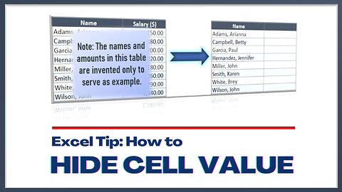
EXCEL TRICK: HOW TO HIDE CELL VALUE
There are data that you don’t want other people like your co-workers who stop by your desk to see. If you are working on a worksheet that contains confidential information like employee salaries, and you don't want others to see, you can hide the contents and make the cells appear blank. Excel has a great way of doing it by applying a number format.
This video presents a tip on how to hide and unhide cell value.
Title: Excel Tip: How to Hide Cell Value
#hidecellvalue
#hideconfidentialinfo
#exceltip
27
views
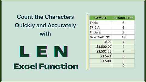
LEN EXCEL FORMULA: COUNTING CHARACTERS MADE EASY
The LEN function in Excel is a very simple but useful tool. It gets the length of text or counts the number of characters in a given text string.
LEN formula returns the number of all characters including space, comma, punctuation and number in a cell, but it does not include number formatting.
The syntax for the LEN function is as follows:
=LEN(text)
where:
text: The cell or text string that you want to count the characters of.
The LEN function can be useful for a variety of tasks, such as checking if a cell or text string is within a certain character limit.
LEN EXCEL FORMULA: COUNTING CHARACTERS MADE EASY
#LENinExcel
#LENExcelFormula
#LENFunction
#HowToCountTheCharactersInExcel
#ExcelFunctions
#ExcelTips
#ExcelTricks
#DataAnalysis
#SpreadsheetTips
#TextManipulation
#ProductivityTips
#ExcelShortcuts
#DataManagement
31
views
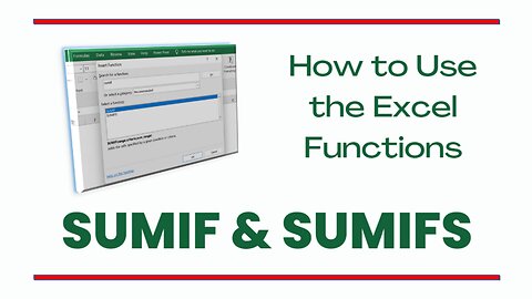
EXCEL SUMIF AND SUMIFS FORMULAS: HOW TO SUM DATA BASED ON CONDITIONS
This video introduces the Excel functions SUMIF and SUMIFS.
The SUMIF formula in Excel is used to sum values in a range based on a single criterion or condition. The syntax for the SUMIF formula is as follows:
=SUMIF(range, criteria, [sum_range])
where:
range: The range of cells that you want to evaluate for the given criteria.
criteria: The condition that must be met in order for the corresponding values in sum range to be included in the sum.
sum range (optional): The range of cells that you want to sum. If this parameter is omitted, the range argument will be used as the sum range.
The SUMIFS formula, on the other hand, allows you to sum values based on multiple criteria. The syntax for the SUMIFS formula is similar to SUMIF, but it allows you to specify multiple criteria in separate ranges. The syntax for the SUMIFS formula is as follows:
=SUMIFS(sum_range, criteria_range1, criteria1, [criteria_range2, criteria2], ...)
where:
sum_range: The range of cells that you want to sum.
criteria_range1: The first range of cells that you want to evaluate for the corresponding criteria.
criteria1: The first condition that must be met in order for the corresponding values in sum_range to be included in the sum.
[criteria_range2, criteria2]: Optional additional ranges and criteria that must be met for the values to be included in the sum.
EXCEL SUMIF AND SUMIFS FORMULAS: HOW TO SUM DATA BASED ON CONDITIONS
#sumif
#sumifs
#sumifexcelformula
#sumifsexcelformula
#sumifinexcel
#sumifsinexcel
#excelsummationbasedoncriteria
#ExcelFormulas
#ExcelTips
#ExcelTricks
#SUMIF
#SUMIFS
#ConditionalSum
#DataAnalysis
#ExcelFunctions
#ExcelShortcuts
#SpreadsheetTips
62
views
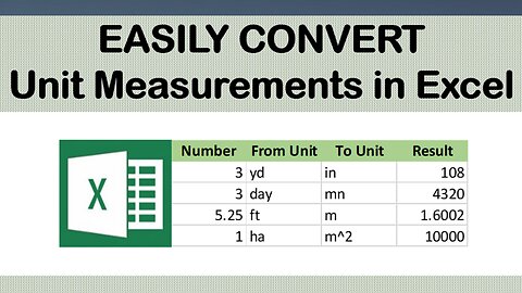
HOW TO USE CONVERT EXCEL FUNCTION FOR VARIOUS UNIT MEASUREMENTS
The CONVERT function in Excel is used to convert a number from one measurement system to another. The syntax for the CONVERT function is:
CONVERT(number, from_unit, to_unit)
where:
Number – The numeric value we wish to convert
From Unit – This is the unit you are converting from
To Unit – This is the unit you are trying to convert to
For example, to convert a value of 10 feet to meters, you can use the formula:
=CONVERT(10, "ft", "m")
This will return the converted value of 3.048 meters.
Watch this video for a complete guide.
HOW TO USE CONVERT EXCEL FUNCTION FOR VARIOUS UNIT MEASUREMENTS
#convert
#ExcelFormulas
#ExcelTips
#ExcelTricks
#ExcelConversion
#ConvertFormula
#MeasurementConversion
#SpreadsheetConversion
#DataConversion
#ExcelFunctions
#ExcelShortcuts
36
views
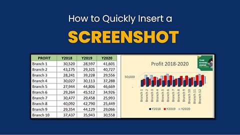
UNLOCK THE MAGIC! HOW TO INSERT A SCREEN CLIPPING IN EXCEL IN SECONDS
This video shows a step-by-step, super-fast and easy procedure to insert a Screen Clipping in Excel.
1. Open the Excel worksheet where you want to insert the screen clipping.
2. Click on the "Insert" tab on the Ribbon.
3. Click on the "Screenshot" button in the "Illustrations" group.
4. From the drop-down menu, select "Screen Clipping". Excel will minimize, and you will see a translucent layer over your screen.
5. Click and drag your cursor to select the portion of the screen you want to capture.
6. Release the mouse button, and the screen clipping will be inserted directly into your worksheet. You can then resize or move the screen clipping as needed.
TIP: You can use a keyboard short-cut to quickly do step 2 to 4. Just press ALT - N - SC - C.
This feature is also available in Microsoft Outlook, PowerPoint, and Word.
TITLE: UNLOCK THE MAGIC! HOW TO INSERT A SCREEN CLIPPING IN EXCEL IN SECONDS
#ExcelTips #ProductivityHacks #ScreenClipping #ExcelShortcuts #DataVisualization #OfficeTips #TechTutorials #Office365 #MicrosoftExcel #InsertScreenClipping #insertpicture #insertreference #shortcutkeys #keyboardshortcuts #spreadsheettips #exceltutorial #excelonline #excelonlinecourse #excelonlinetraining #datavisualization #learnexcel #excelforbeginners #excelhacks #excelspreadsheets
43
views
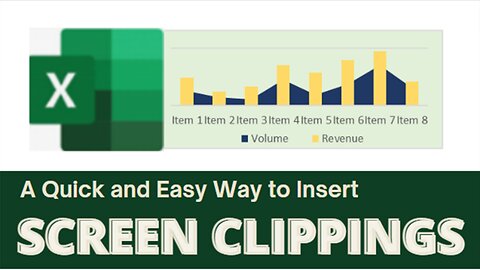
MASTERING EXCEL: INSERTING SCREENSHOTS LIKE A PRO
A picture is worth a thousand words. Similarly speaking, a screenshot can speak a thousand words. Therefore, this can be a perfect addition to your Excel spreadsheet.
A screenshot can also be a good reference for your numbers in excel. It can be an excerpt from an email. Having the reference in one window is a lot easier as you will be able to capture information without leaving the program that you are working in. You can also add a graph or chart from other files for better illustration or presentation of your data.
If you are going through a long process when you add screenshot to your Excel or Office file, I have good news for you. There’s a quick and easy way to do that, with the use of the function Screenshot. It is useful for capturing snapshots of programs or windows that you have open on your computer.
This feature is available in Excel, Outlook, PowerPoint, and Word but our example here will be on Excel.
Screenshot is a great tool that can quickly add images from the other open windows and it’s so easy to do.
Title: Mastering Excel - How to Insert Screenshots Like A Pro
#ExcelTips
#ExcelTricks
#ExcelTutorial
#ExcelScreenshot
#ExcelInsertScreenshot
#ExcelHowTo
#ExcelTraining
#ExcelBeginner
#ExcelIntermediate
#ExcelExpert
#ExcelFunctions
#ExcelFormulas
#SpreadsheetTips
#SpreadsheetTricks
#SpreadsheetTutorial
#SpreadsheetTraining
#SpreadsheetHowTo
#DataVisualization
#ProductivityHacks
#MicrosoftOffice
47
views
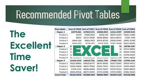
EXCEL TUTORIAL: QUICKLY ORGANIZE DATA WITH RECOMMENDED PIVOT TABLES
A pivot table is a table of grouped values that aggregates the individual items of a more extensive or detailed data set or spreadsheet into one or more categories. It groups the data together using a chosen aggregation function. It is one of Excel’s most valuable features. And Excel makes it easier for us to have a Pivot Table by introducing Recommended Pivot Tables.
In this video, you will learn how to use the Recommended Pivot Tables feature to quickly and easily summarize large sets of data. We will cover how to create a pivot table using Recommended Pivot Tables, customize the layout and format of the pivot table, and utilize powerful features such as filtering, sorting, and grouping to analyze data in meaningful ways. Whether you're a beginner or an experienced Excel user, this tutorial will provide you with the knowledge and skills to efficiently manage and analyze data in MS Excel.
Title: Quickly Organize Data with Recommended Pivot Tables
#Excel #PivotTable #DataAnalysis #RecommendedPivotTables #DataVisualization #MicrosoftOffice #Spreadsheet #BusinessIntelligence #DataManagement #Productivity #ExcelTips #ExcelTricks #DataSummarization #DataReporting #TimeSavingExcelFunction #ExcelTutorial #LearnExcel #ExcelOnline #ExcelTraining
69
views
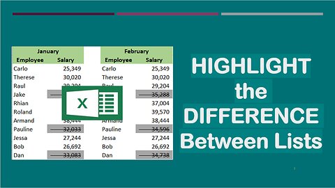
DIFFERENCE BETWEEN LISTS: HOW TO IDENTIFY AND HIGHLIGHT UNIQUE VALUES IN EXCEL
There are different ways to identify differences between lists. This video shows a method that will not only identify differences but will also format the differences or the unique values found. This can be quickly done even if the lists contain large amounts of data.
The Excel function presented here is Conditional Formatting under the Home tab. This is useful when you want to identify any changes, like if you want to know the employees who were given salary increase in a particular month. With the use of Conditional Formatting New Rule, you can easily get this information. And there’s a keyboard shortcut that can quickly bring you to the New Formatting Rule window.
Watch this video for a complete guide.
Title: Difference Between Lists: How to Identify and Highlight Unique Values in Excel
#ExcelTutorial
#LearnExcel
#ExcelFunctions
#ExcelSkills
#DifferenceBetweenLists
#IdentifyAndHighlightChanges
#IdentifyDifferenceBetweenLists
#HighlightDifferenceBetweenLists
#HighlightUniqueValues
#ConditionalFormatting
#ConditionalFormattingNewRule
#FormatOnlyUniqueValues
#HowToIdentifyAndHighlightDifferencesBetweenLists
#ShortcutKeys
#KeyboardShortcuts
35
views

IFERROR - THE ORGANIZED WAY TO HANDLE FORMULA ERRORS
IFERROR is an easy and organized way to trap and handle formula errors . Watch this video to see how this is being done.
Sometimes, your formula returns an error. There are various types of errors such as:
-When you try to divide a number by zero
-When you use a VLOOKUP function and the value is not available
-An error when a formula refers to a cell that’s not valid
-A calculation error
-An error when the formula cannot recognize something in it like if you used the wrong formula name
If you don’t want such errors to appear in your spreadsheet or report, Excel can return or display a friendly message as an alternative to notify about the error. The IFERROR function can help you with it. It’s an elegant way to trap and manage errors without using more complicated nested IF statements. IFERROR function returns a custom result when a formula generates an error, and if no error is detected, it simply returns the standard result of the formula.
Title: IFERROR - The Structured Way to Handle Errors in Excel
#TheExcelZone
#ExcelTipsAndTricks
#ExcelShortcuts
#MicrosoftExcel
#AdvancedExcelTutorial
#ExcelOnlineTraining
#ExcelOnlineCourse
#Excel365
#Office365
#LearnExcel
#HelpfulExcelFunctions
#IFERROR
#ExcelFormula
#HowToHideErrors
#SetNotificationInsteadOfError
55
views

IFS EXCEL FUNCTION: THE EASIER WAY TO DO MULTIPLE CONDITIONS
This video introduces the easier way to do the IF function with multiple conditions compared to the Nested IF Statement in my previous video. It’s through the IFS function available in Excel 2019 and Office 365.
Similar to the NESTED IF STATEMENT, the first step to do the IFS function is to define our goal for the given data. Once we have the goal, we can easily fill out the IFS formula. The basic guide is indicate IF, then the logical test 1 followed by value 1, test 2 followed by value 2 and so on. Just like the Nested IF Statement, we should make sure that the formula covers all potential conditions and scenarios.
And you just learned how to use the IFS function. Practice if you need to in order to have a strong level of confidence around logical structuring.
Title: IFS Excel Function: The Easier Way to Do Multiple Conditions
#ifsexcelfunction
#easierwaytodomultipleconditions
#logicaltest
#multipleconditions
57
views

EXCEL TUTORIAL: MASTERING THE IF FUNCTION FOR DATA ANALYSIS - HOW TO SET MULTIPLE CONDITIONS
The IF function is a logical function in Microsoft Excel that allows users to test a condition and return one value if the condition is true, and another value if the condition is false. The basic syntax of the IF function is as follows:
=IF(logical_test, value_if_true, value_if_false)
Here's what each part of the syntax means:
logical_test: This is the condition that you want to test. It can be any logical expression that evaluates to either TRUE or FALSE. For example, you could test whether a cell contains a certain value, whether one cell is greater than another, or whether a date is before or after a certain date.
value_if_true: This is the value that Excel will return if the logical_test is TRUE. It can be a number, text, or any other type of value that you want to display if the condition is met.
value_if_false: This is the value that Excel will return if the logical_test is FALSE. Again, it can be any type of value that you want to display if the condition is not met.
For example, suppose you have a spreadsheet that tracks students' grades, and you want to display whether each student passed or failed based on whether their grade is above or below 60. You could use the following formula in a new column to display "Pass" or "Fail" based on each student's grade:
=IF(B2>=60, "Pass", "Fail")
In this formula, B2 is the cell that contains the student's grade. If the grade is greater than or equal to 60, the formula will return "Pass". Otherwise, it will return "Fail".
The IF function can be nested within other functions to create more complex logical tests, and it can be combined with other Excel functions to perform calculations and manipulate data based on certain conditions.
Title: Mastering the If Function for Data Analysis - How to Set Multiple Conditions
#ExcelTips #ExcelFunctions #ExcelFormulas #IFFunction #LogicalFunctions #IfExcelFunction #IfWithMultipleConditions #DataAnalysis #DecisionMaking #ProductivityTools #SpreadsheetTips #ExcelTutorials #SpreadsheetFunctions #ConditionalStatements #ExcelTricks #MicrosoftExcel #ExcelExperts #DataManipulation #OfficeTips #SpreadsheetHacks #AutomationTools #BusinessProductivity #ExcelShortcuts #DataVisualization
55
views
EXCEL TUTORIAL: AUTO-COPY FUNCTION TO SAVE TIME
In Excel, Auto-copy is a feature that allows you to automatically copy a cell's formula to the adjacent cells when you double-click the cell's fill handle (the small square in the lower right corner of the cell).
Auto-copy can help save time when you need to create a series of formulas. Instead of manually copying and pasting the formulas, you can simply double-click the fill handle and let Excel do the work for you.
Watch this video for a detailed tutorial.
Title: Auto-copy Excel Function to Save Time
#ExcelTutorial #AutoCopy #ExcelTips #ProductivityHacks #SpreadsheetSkills #DataManagement #AutomateTasks #TimeSaver #EfficientExcel #ExcelTricks #LearnExcel #OfficeSkills #MicrosoftExcel #CopyPasteTricks #CopyAutomation #DataCopying #ExcelShortcuts #DataEntryMadeEasy #AutomationTutorial #SpreadsheetTutorial
27
views

EXCEL TUTORIAL: FLASH FILL - THE SUPER TIME-SAVING TOOL
Excel's Flash Fill function is a great tool that allows you to quickly and easily fill in values, split text, concatenate data, and more, saving you time and effort when working with large datasets.
How Does Flash Fill Work?
Flash Fill uses pattern recognition to analyze the data you're working with and do transformations based on the pattern it identifies. To use Flash Fill, simply start typing the transformation you want to apply to your data in a new column next to the original data. Excel will automatically fill the succeeding cells with the same pattern.
Benefits of Flash Fill
The Flash Fill function in Excel is a useful tool that can save you a lot of time and effort when working with large datasets. By automating repetitive data transformations, you can focus on analyzing and interpreting your data, rather than spending hours manually doing it.
Flash Fill can also help ensure data accuracy by reducing the risk of human error. When you use Flash Fill to automatically apply transformations to your data, you can be confident that your results are accurate and consistent. Flash Fill can help you get the job done quickly and efficiently.
Title: Flash Fill - The Time-Saving Excel Tool
#ExcelTutorial #FlashFill #ProductivityTips #DataCleaning #ExcelTips #DataTransformation #SpreadsheetTricks #OfficeTips #ExcelFunctions #ExcelTraining #ExcelForBeginners #ExcelForProfessionals #AutomaticEntryOfData #ExtractDataFromAnotherCell #AmazingExcelTool #ExcelOnline #ExcelFunction #KeyboardShortcut
32
views
MASTERING EXCEL: HOW TO USE AUTO FILL TO STREAMLINE YOUR DUTY
Auto Fill is an Excel feature that allows you to automatically fill a series of cells with a particular pattern or sequence of data. This can be a real time-saver, especially when working with large sets of data.
To use the Auto Fill function, follow these simple steps:
1. Start by entering the data or formula that you want to repeat in the first cell of the series.
2. Click and drag the small square located in the bottom right corner of the cell to the end of the range where you want the data to be filled.
Excel will automatically fill the selected cells with the pattern or sequence that you started with.
Auto Fill also has other features that can help to customize the data sequence. For example, you can use the fill handle to drag the selection horizontally or vertically. You can also use the Auto Fill Options button that appears after you fill the cells to choose a different fill type or to copy only the values without the formulas.
In addition to making data entry more efficient, Auto Fill can also help to reduce errors and ensure consistency in your data. By automating the data entry process, you can avoid the potential for human error that can occur when manually entering data or copying and pasting data between cells.
In conclusion, Auto Fill is a valuable tool for anyone who works with large sets of data in Excel. It can help to streamline the data entry process, reduce errors, and ensure consistency in your data. So, the next time you need to fill in a series of cells, give Auto Fill a try and see how it can save you time and improve your productivity.
Title: Mastering Excel - How to Use Auto Fill to Streamline Your Duty
#ExcelAutoFill #AutoFillFunction #DataEntryAutomation #ExcelTips #ExcelTricks #ProductivityHacks #EfficiencyBoost #DataManipulation #DataAnalysis #SpreadsheetSkills #ExcelFormulas #SpreadsheetTips #DataVisualization
39
views
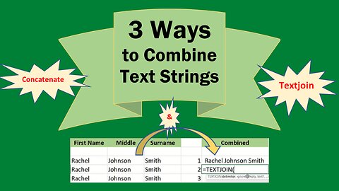
EXCEL TUTORIAL: 3 WAYS TO COMBINE TEXT STRINGS
If you want to combine two or more text strings and place them together in one cell, there are three ways to do that:
1. With the use of the Concatenate Excel formula.
2. Through the Textjoin Excel formula which concatenates a list or range of text strings using a delimiter.
3. Combine text strings using &.
The complete guide for the three methods to combine or concatenate data is presented in this video.
Title: Excel Tutorial: 3 Ways to Combine Text Strings
#exceltipsandtricks
#excelshortcuts
#microsoftexceltutorial
#advancedexceltutorial
#excelonlinecourse
#excel365
#exceltipstricksandshortcuts
#bestexcelshortcuts
#learnexcel
#exceltraining
#excelformulasandfunctions
#microsoftexceltips
#exceltipsandtricks
#keyboardshortcuts
#excelfunctions
#combinetextstrings
#concatenateexcel
#textjoin
#concatenatetextstrings
#combinetexts
43
views
EXCEL TUTORIAL: HOW TO CONSOLIDATE DATA WITH KEYBOARD SHORTCUT
This video features an excel function that is used to consolidate data from one workbook, or from different open workbooks. You can simply click ALT-A-N and you will be directed to the consolidate window. You can also find it under the data tab.
To consolidate data from 1 sheet, click the keyboard shortcut ALT-A-N. Use the default function sum, but you can change it if you want to do other functions from the drop-down list like count, average, max, min and many others. Then input the reference. Below that says, use labels in, and choose left column. And you will have the consolidated figures.
If you do consolidation of data from different sheets, you still have to click the same keys, Alt-A-N, click the reference box and select the amounts in Sheet 1 as the first reference. Click add, and the first reference is added to all references box. Put the cursor back to the reference box and choose the numbers from sheet 2 as the 2nd reference, then click add again and it’s transferred to all references. Then repeat the process for the 3rd reference and do the same for the succeeding references if any.
There’s more. If you want to show the links or the sources of the data, you can tick “create links to source data”.
Title: How to Consolidate Data in Excel
#exceltipsandtricks
#exceltipsandtricks
#exceltips
#tricksandshortcuts
#excelshortcuts
#excel
#microsoftexcel
#advancedexceltricks
#excelonlinecourse
#exceltipstricksandshortcuts
#exceltutorial
#bestexcelshortcuts
#learnexcel
#exceltraining
#excelformulasandfunctions
#microsoftexceltips
#keyboardshortcuts
#excelfunctions
#consolidatedatainexcel
#consolidate
#howtoconsolidatedatainexcel
#bestexcelformulas
#consolidateexcelfunction
58
views
3 WAYS TO SHOW AND HIDE FORMULAS IN EXCEL
If you want to review a formula of one cell, you can just simply click the cell and the formula appears at the formula bar. You can also double click the cell or click f2 and the formula appears in that cell. But this is not applicable if you have to check the formula of several cells. No problem. Excel has built-in tools that you can use to display them simultaneously. This video presents the ways to show and hide formulas.
Title: 3 Ways to Show and Hide Formulas in Excel
#keyboardshortcuts #exceltutorial #showformulas #hide formulas
28
views
INSTANTLY FIND AND SELECT DATA WITH EXCEL'S ADVANCED SELECT FUNCTION
Make use of the Advanced Select Excel function with super easy steps. You just need 3 combinations of keyboard shortcuts, and you have the data selected and highlighted. This is such an efficient way to find and select data.
Title: Instantly Find and Select Data with Excel's Advanced Select Function
#advancedselect #findandselectdata #exceltutorial #keyboardshortcut
27
views

MS EXCEL TUTORIAL: TIPS TO QUICKLY HIGHLIGHT THE CELLS AND NAVIGATE THE TABS
Highlighting cells in Excel can be much faster using some simple shortcut keys. You can quickly select and highlight multiple cells in a contiguous range with the use of 3 shortcut keys – control, shift and arrow.
Watch this video to know how. Plus you will also learn how to swiftly navigate the tabs without using a mouse.
TITLE: TIPS TO QUICKLY HIGHLIGHT CELLS AND NAVIGATE THE TABS
#exceltutorial #excelkeyboardshortcut #exceltips #quicklyhighlightcells #quicklynavigatethetabs
32
views